A Base case, an Upside case and a Downside case can create a false sense of coverage. Suppose a company starts with 30 units of usable cash, treats 8 as its minimum cash boundary, and sees its ordinary Downside bottom at 11. Nothing in that Downside breaches the line.
That result is useful, but narrower than it looks. It says one chosen path survives. It says nothing about a combination in which demand weakens, realised price falls and collections slow at the same time. It also says nothing about whether management can act quickly enough if the cash path turns.
The synthetic company below is designed to answer those harder questions. The numbers are teaching data, not observations from a real business. The aim is to connect five methods that are often collapsed into one spreadsheet exercise: Forecast, Scenario, Sensitivity, Stress Test and Reverse Stress Test.
A forecast is one path, not the uncertainty map
A Forecast is the expected path under the information available today. That is already a substantial job. It does not also need to represent every alternative future, every decision boundary and every way the business might fail.
| Method | Practical job |
|---|---|
| Forecast | State the current expected path |
| Scenario | Build an alternative path from linked assumptions |
| Sensitivity | Isolate how one or a few drivers move the result |
| Stress Test | Test survivability under a deliberately adverse hypothetical state |
| Reverse Stress Test | Define failure, then identify combinations capable of causing it |
The troublesome overlap is between a Downside and a Stress Test. The US Federal Reserve explicitly labels its supervisory stress scenarios as hypothetical scenarios, not forecasts. Corporate finance does not inherit the Fed’s regulatory framework, but the distinction is useful: a stress scenario is constructed to reveal vulnerability, not to win a contest for the most likely bad forecast.
A Forecast multiplied by three percentages can produce three neat tabs. It still leaves the uncertainty model largely untouched.
A downside scenario must move linked assumptions together
Consider this operating setup:
| Driver | Baseline | Ordinary Downside | Severe Stress |
|---|---|---|---|
| Demand / volume index | 100 | 90 | 82 |
| Realised price / mix index | 100 | 97 | 94 |
| Gross margin | 45% | 40% | 35% |
| Collection timing / DSO | 45 days | 60 days | 75 days |
| Fixed-cost response | Not required | Begins after 6 weeks | Begins after 6 weeks, limited initial effect |
The ordinary Downside changes more than sales. Weaker demand is accompanied by a softer realised price/mix, lower gross margin and slower collections. Fixed cash costs do not adjust immediately. The resulting path has an operating story rather than a single edited cell.
That coherence is the reason to separate Scenario from Sensitivity. A one-way Revenue -10% test is perfectly legitimate when the question is local. It becomes misleading only when the organisation treats that local movement as a complete alternative state of the business.
The TCFD scenario-analysis material offers useful methodology here even though it was written for climate-related risk. Its value is the discipline of internally consistent assumptions and linked drivers. Nothing in that transfer turns climate-disclosure requirements into a general corporate-finance obligation.
Probability can wait. Before estimating how likely an alternative path might be, management can learn a great deal by asking where the decision itself changes.
Find the value that flips the decision
The baseline six-month cash trough is 18. Management has also decided that a projected trough below 12 is enough to begin contingency preparation. The company is not yet at its minimum cash boundary of 8; it is simply close enough that waiting has become an active choice.
Hold other assumptions at baseline and the sensitivity analysis gives two useful markers. A realised price/mix index of roughly 95, down from 100, brings the projected trough towards 12. So does a DSO of roughly 63 days, up from 45 days.
These are switching values. They measure how far the current plan sits from a decision change. They do not tell us how probable either movement is. The UK Department for Transport’s uncertainty toolkit uses the same idea as a robustness test: identify the point at which the conclusion changes, then examine the distance to that point.
This distinction matters beyond sensitivity charts. Accounting break-even can coexist with a liquidity problem if cash arrives too late. A P&L that still looks tolerable therefore cannot settle the survivability question on its own.
A stress test asks whether the business survives the adverse path
The severe path combines the adverse movements rather than testing them one by one. Basel Committee stress-testing principles emphasise adverse conditions, material risks and scenario consistency. Those principles come from banking supervision; here they are used only as methodological discipline.
The cash result is more revealing than the revenue result:
| Point in time | Baseline | Ordinary Downside | Severe Stress |
|---|---|---|---|
| Opening | 30 | 30 | 30 |
| Month 1 | 28 | 26 | 24 |
| Month 2 | 26 | 22 | 19 |
| Month 3 | 23 | 17 | 13 |
| Month 4 | 21 | 14 | 7 |
| Month 5 | 19 | 11 | 6 |
| Month 6 | 18 | 12 | 9 |
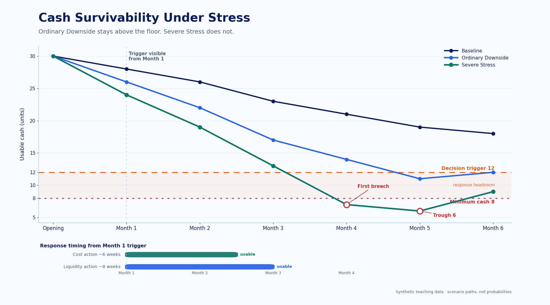
Under the ordinary Downside, usable closing cash never falls below 11. Severe Stress crosses the minimum cash boundary of 8 in Month 4 and reaches 6 in Month 5.
The word usable matters. Headline cash may include money that is restricted, trapped in another legal entity, committed to near-term payments or operationally unavailable. Runway should be built from resources that can actually be deployed when required. The minimum-cash boundary also belongs to the company, not to a universal formula. 8 is an illustrative operating and risk boundary here, not a standard number of months of burn.
Timing then becomes decisive. The cost plan takes about 6 weeks before it materially improves cash. A liquidity action takes about 8 weeks from formal start until the additional funds are usable. If the model waits until cash is already at 8 before assuming action, it has quietly granted management time it does not have.
That is why a 13-week cash view is more informative under pressure than a historical average burn calculation. AFP and Deloitte treasury material both focus on forward cash timing and dated events. In this case the result is unambiguous: without additional liquidity intervention, the adverse path crosses 8 in Month 4 and reaches a trough of 6 in Month 5.
One severe path, however, is still only one path.
Reverse stress starts from failure and works backward
For reverse stress, the company does not first choose another severe scenario. It defines failure:
Usable cash falls below 8 before the planned liquidity action can become effective.
Management is assumed to trigger the liquidity action at the end of Month 1. With an 8-week lead time, funds are available around the beginning of Month 4. The reverse-stress task is therefore to find driver combinations that push cash below 8 before then.
The model produces several examples:
| Combination | Volume | Price / mix | DSO | Cost-action delay | Month 3 usable cash |
|---|---|---|---|---|---|
| A | 80 | 94 | 72 days | 6 weeks | 7.6 |
| B | 84 | 96 | 88 days | 6 weeks | 7.8 |
| C | 86 | 93 | 68 days | 10 weeks | 7.5 |
Combination A gets there with deeper volume weakness. B relies more heavily on collections. C combines price pressure with a 10-week delay in the cost response. None of those rows is a probability statement. Each is simply sufficient, in this model, to cross the failure boundary before the planned response can take effect.
PRA and EBA reverse-stress material comes from prudential regulation. The transferable idea is the failure-first direction of travel: define when the business model becomes unviable, then work backwards to the conditions that cause it. The regulatory obligation itself does not transfer to every company.
This also exposes a weakness in the phrase “we tested our worst case”. Passing one selected aggregate stress case cannot prove that no nearby combination fails earlier.
A boundary needs a trigger, owner and action
The cash boundary is 8, but waiting for 8 would make the 8-week liquidity lead time largely useless. The company therefore needs a management trigger that sits ahead of failure.
In this example that trigger is 12, observed through the 13-week projected usable closing cash forecast. At the end of Month 1, the severe path already shows the next 13 weeks falling below 12, so management starts the prepared response then.
| Field | Design |
|---|---|
| Observable signal | 13-week projected usable closing cash |
| Trigger threshold | Below 12 |
| Severe-path trigger timing | At the end of Month 1, the next 13 weeks already project cash below 12 |
| Owner | CFO, with Finance owning the cash forecast and Operations owning the cost action |
| Liquidity action | Start the pre-prepared liquidity package immediately, targeting 7 additional units of usable funding |
| Cost action | Start the pre-agreed cost plan, improving monthly cash by 1.5 after roughly 6 weeks |
| Liquidity lead time | About 8 weeks |
| Prerequisites | Current 13-week forecast, board approval path, lender/investor data pack, collection action list |
| Escalation | If projected cash falls below 10, or the action schedule slips by more than 1 week, escalate to CEO + Board / Finance-Risk forum |
| Expected effect | Add liquidity headroom before Severe Stress crosses 8, then reduce monthly cash burn |
The separation between 12 and 8 is intentional. 8 is the failure boundary; 12 is a decision boundary shaped by execution time. It is not offered as a universal liquidity rule.
Several pieces of the model meet here. Sensitivity identified where the decision flips. The forward cash forecast showed the time remaining. Liquidity planning supplied the lead time. Governance determines ownership and escalation. The FRC’s guidance on agreed escalation triggers is a useful analogue for that last piece, but its formal setting is UK corporate governance, not a universal legal requirement.
A contingency plan also needs more than labels. “Raise capital”, “refinance” or “cut costs” do not become executable because they appear in a spreadsheet cell. The owner, prerequisites, timing and route to execution are part of the financial model whenever delay can determine survival.
Calibrate the next cycle with forecast error, not permanent ±10% ranges
Actual results should change the next set of assumptions. Otherwise a Scenario framework slowly turns into ritual: the same ±10% survives every planning cycle regardless of where the Forecast is actually wrong.
The feedback loop is straightforward:
forecast → actual → error / bias / calibration → update driver ranges and scenario assumptions → rerun switching values / stress / triggers
Suppose collection timing repeatedly comes in slower than forecast. That is evidence to revisit the DSO baseline and downside range, not merely a reason to widen revenue. If demand is broadly unbiased while realised price/mix is consistently optimistic, uncertainty should be concentrated where the model is demonstrably miscalibrated.
Forecast accuracy itself needs care. Hyndman and Koehler show that MAPE can behave badly when actual values are zero or close to zero. Evaluation should also be genuinely out of sample; accuracy measured on data already used to fit the model is not the same test.
A probabilistic Forecast raises a different evaluation problem. Prediction intervals and quantiles need interval, quantile or other distribution-aware checks; a midpoint error cannot establish calibration of the whole distribution. Even then, Base / Upside / Downside labels do not gain probabilities automatically. A genuine probability distribution requires separate probabilistic modelling and evidential support.
In practice, the recurring management routine can stay compact. Keep the current expected path visible. Know which linked assumptions define the alternatives. Track the values that change the decision. Watch the cash trough against minimum usable cash. Know which combinations can beat the response time, and trigger action early enough to matter. Then use actual forecast errors to alter the next cycle rather than preserving yesterday’s ranges by habit.
That is the useful end state of Scenario work: not a collection of increasingly pessimistic tabs, but a model that tells management where the boundary is and whether there is still time to act.
References
- Basel Committee on Banking Supervision, Stress testing principles (2018): https://www.bis.org/bcbs/publ/d450.pdf
- Board of Governors of the Federal Reserve System, 2026 Stress Test Scenarios: https://www.federalreserve.gov/publications/2026-stress-test-scenarios.htm
- Task Force on Climate-related Financial Disclosures, The Use of Scenario Analysis in Disclosure of Climate-Related Risks and Opportunities (2017): https://www.fsb-tcfd.org/wp-content/uploads/2017/06/final-tcfd-technical-supplement-062917.pdf
- UK Department for Transport, TAG Uncertainty Toolkit (2026): https://assets.publishing.service.gov.uk/media/6a185b32050971fbebf3bbf3/tag-uncertainty-toolkit-May-2026.pdf
- Bank of England Prudential Regulation Authority, SS31/15: The Internal Capital Adequacy Assessment Process and Supervisory Review: https://www.bankofengland.co.uk/prudential-regulation/publication/2013/the-internal-capital-adequacy-assessment-process-and-supervisory-review-ss
- European Banking Authority, Guidelines on stress testing: https://www.eba.europa.eu/activities/single-rulebook/regulatory-activities/supervisory-review-and-evaluation-process-srep-and-pillar-2/guidelines-stress-testing
- Association for Financial Professionals, Cash Forecasting: A Free Cash Flow Perspective (2022): https://www.afponline.org/docs/librariesprovider2/default-document-library/122-cash-forecasting-a-free-cash-flow-perspective.pdf
- Association for Financial Professionals, Keeping the Lights On: The Why and How of Liquidity Management: https://www.afponline.org/topics/treasury/keeping-the-lights-on-the-why-and-how-of-liquidity-management
- Deloitte, 13-Week Cash Flow Forecasting (2020): https://www2.deloitte.com/ro/en/pages/finance/solutions/13-week-cash-flow-forecasting.html
- Financial Reporting Council, Corporate Governance Code Guidance: https://www.frc.org.uk/library/standards-codes-policy/corporate-governance/corporate-governance-code-guidance/
- Hyndman & Athanasopoulos, Forecasting: Principles and Practice, 3rd ed.: https://otexts.com/fpp3/
- Hyndman & Koehler, Another Look at Measures of Forecast Accuracy (2006): https://robjhyndman.com/papers/mase.pdf