Imagine a B2B SaaS company preparing its forecast for next quarter.
Revenue in the same quarter last year was 100 million. Sales still feels reasonably positive about demand, so management starts with a familiar shortcut: last year plus 10%. The team takes 110 million, spreads it across three months and allocates the total to product lines. Nothing looks obviously wrong on the spreadsheet.
A month later, several inputs have moved. Qualified pipeline is below plan. Win rate has not collapsed. A few large deals have slipped. Churn is higher than assumed. Two sales hires that were due to start this month will arrive two months late.
Finance can see the miss. The spreadsheet cannot yet explain it. The useful questions are more specific: did demand weaken, did conversion move, did retention deteriorate, did pricing shift, or did the business simply have less capacity than the plan assumed?
A forecasting process earns its place in management when those questions can be answered from the model rather than reconstructed after the fact.
Start with a mechanism you can inspect
Multiplying last year’s revenue by 1.10 is mathematically straightforward. The difficulty is informational: one top-line growth rate can hide several different operating stories. An 8% revenue miss, for example, could come from a 15% pipeline shortfall with better-than-expected win rate, a lower average contract value, higher churn, delayed sales capacity, or revenue timing moving into the next period.
This is why IMA’s FP&A work is useful here. It links financial outcomes to operating drivers so managers can understand how the result was formed. Its managerial-costing guidance makes a related argument around resource consumption and causal relationships rather than convenient allocation bases. For forecasting, the practical test is whether a proposed driver has a plausible operating mechanism that connects it to the output.
Correlation alone does not settle that question. A KPI may move with revenue and still be a poor driver if no one can explain what action or resource relationship sits between the two.
A simple diagnostic is to ask: if this input changes, what happens next in the business, and why should that alter the financial result?
Give each input a clear role
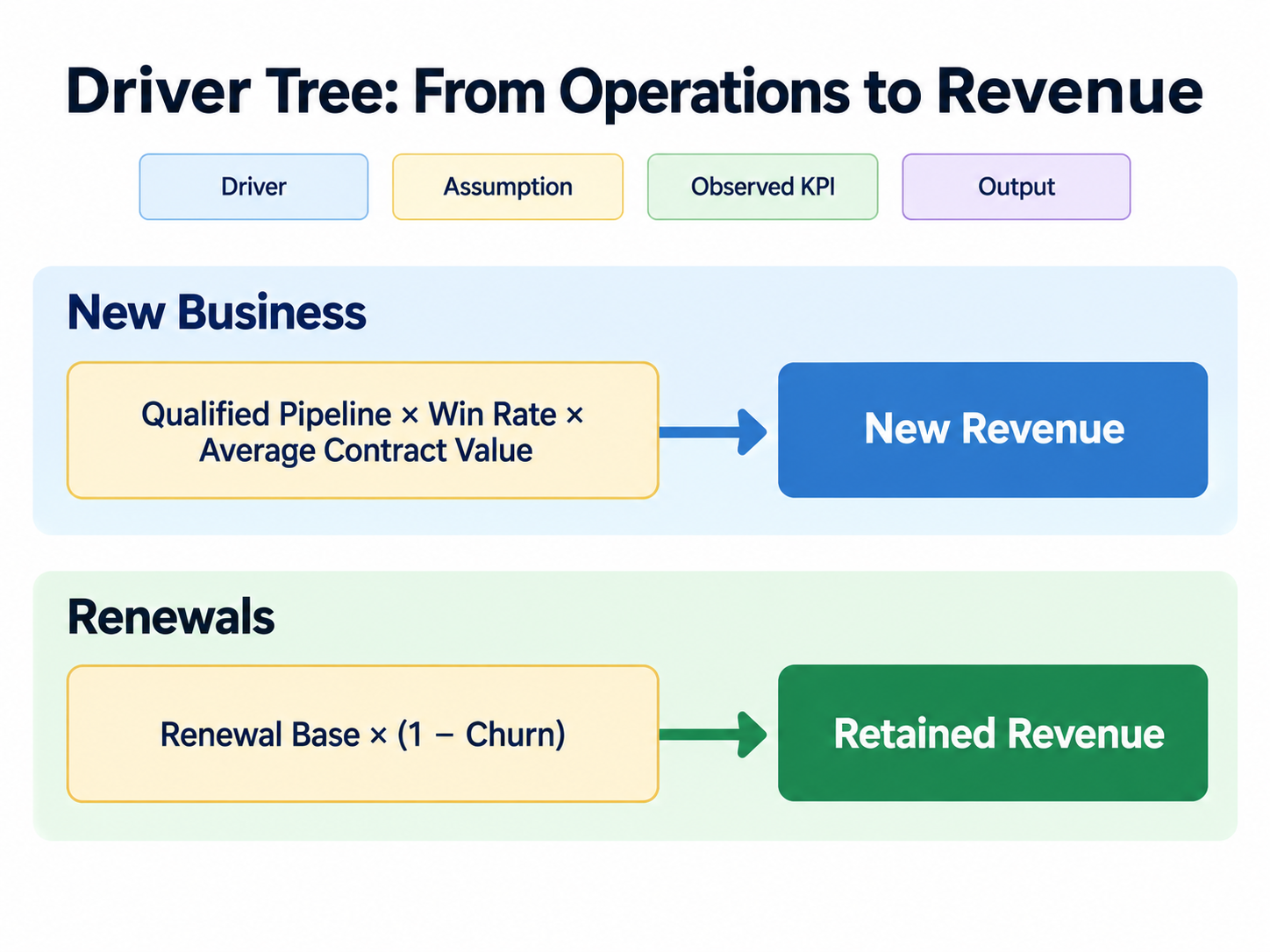
Four labels prevent a surprising amount of confusion: Driver, Assumption, Observed KPI and Output. A Driver represents an operating mechanism such as qualified pipeline, win rate, churn or ramped sales capacity. An Assumption is the value currently fed into that mechanism, for example a 22% quarterly win rate or 1.5% monthly churn. An Observed KPI records what the business has actually measured, such as pipeline coverage or realised churn. The Output is what the model calculates: new ARR, retained revenue, Opex or cash burn.
For new revenue, the model might begin with:
Qualified Pipeline × Win Rate × Average Contract Value → New Revenue
Retained revenue can use:
Renewal Base × (1 − Churn) → Retained Revenue
The same approach works on capacity and cost:
Sales Headcount × Ramped Productivity → Sales Capacity
Engineering Headcount × Loaded Cost → Engineering Opex
Cloud Usage × Unit Infrastructure Cost → Infrastructure Cost
These equations are illustrative, not a standard SaaS model. Their job is to expose the relationship between an operating input and a financial output so that the relationship can later be tested.
GFOA’s planning guidance is written for public finance, but one element transfers cleanly: distinguish leading from lagging drivers and make the decision horizon explicit. In a corporate model, that means being clear about which signal moves first, which result follows, and over what period.
Visibility matters just as much as the formula. A 22% win-rate assumption buried in a hidden cell, hiring dates silently copied from last year, or churn hard-coded in an unowned tab leaves the model difficult to challenge. ICAEW’s spreadsheet principles emphasise visible inputs, assumptions and logic. The Federal Reserve and OCC’s model-risk guidance is much heavier and belongs to regulated financial institutions, but its principle of challenging material assumptions is still relevant when used with that boundary in mind.
For ordinary FP&A, four pieces of context are usually enough to make an assumption discussable: its current value, the evidence or judgement behind it, the last update date, and the person expected to challenge it when conditions change.
Keep the planning window moving
A driver model loses relevance at different speeds. Pipeline may change quickly; office rent may not. Before choosing an update schedule, define how far forward management needs to see.
AICPA & CIMA describe a rolling plan as a planning window that moves forward as periods close. If management always wants six quarters of visibility, the first view might cover Q1–Q6. Once Q1 closes, Q1 becomes actual and Q7 is added. The view is now Q2–Q7. A quarter later it becomes Q3–Q8.
That is the rolling horizon. Refresh cadence is a separate design choice.
AFP’s guidance treats horizon, time increments and update design as company-specific. Its implementation material also warns about recreating the full annual-budget workload four or twelve times a year. More frequent work does not automatically create better information.
The cadence should reflect the decision environment. A hiring decision that must be made next quarter needs the headcount driver early enough to matter. A volatile pipeline may justify frequent review, while office rent will usually move more slowly. Data also has its own maturity: a signal that becomes reliable monthly does not become more informative because the dashboard refreshes every day. Materiality sets another threshold, and the cost of involving Finance, Sales, Ops and management belongs in the design as well.
The result can be deliberately uneven. Some drivers may be monitored weekly and reforecast monthly; slower costs may be reconsidered quarterly; the six-quarter horizon can remain unchanged throughout.
Annual Budget can still coexist with this process. Ekholm and Wallin found that flexible and rolling instruments can complement annual budgeting. The detailed division of labour between AOP, Budget and Forecast belongs elsewhere; for this article, the relevant point is simply that rolling the forward view does not require throwing away the annual planning process.
Save the old forecast before reality arrives
Forecast evaluation becomes misleading when each revision replaces the previous version.
Take a simple sequence. In January, the company forecasts March revenue at 30 million. In February, new information brings the forecast down to 27 million. The March actual is 26.8 million. Comparing only the late-February forecast with the actual produces a miss of 0.2 million.
That is a valid measurement of the late-February view. It says nothing about the quality of the January two-month-ahead forecast.
The missing piece is the forecast origin: when the forecast was made, what information was available then, and how far ahead the estimate reached. Hyndman and Athanasopoulos distinguish genuine forecast errors from residuals calculated on data the model has already seen. For management, the rule is straightforward. Judge the January forecast using the January information set.
The SaaS example therefore needs a stored January snapshot of qualified pipeline, the win-rate assumption, the churn assumption, expected sales hiring and ramp, and the resulting revenue and cost outputs. February and March actuals can then be compared with what the business genuinely believed in January.
This also exposes horizon effects. One-month-ahead forecasts may be stable while three-month-ahead forecasts begin to drift and six-month-ahead estimates lose most of their decision value. A single statement such as “forecast accuracy is 87%” cannot show that pattern.
Diagnose error from more than one angle
Once genuine prior forecasts have been preserved, accuracy can be analysed without pretending that one metric answers every management question.
Size of the miss
MAE, or mean absolute error, keeps the result in the original unit. Revenue error remains a monetary amount; headcount error remains a number of people. RMSE gives relatively more weight to large misses, which can be useful when occasional large errors are particularly damaging. The choice depends on what kind of miss matters to the decision.
Direction of the miss
A business can have a respectable aggregate MAE while repeatedly overestimating one driver. If win rate has been too high for several months, the pattern deserves attention even when positive and negative revenue errors partly offset each other.
Sales may consistently rate late-stage pipeline too optimistically. Finance may systematically understate revenue in the name of conservatism. Similar average error does not imply the same organisational problem.
Distance from the forecast origin
Hyndman and Athanasopoulos use rolling forecast origins in time-series cross-validation to examine how error changes with horizon. The management adaptation is simple: keep one-month-ahead, three-month-ahead and six-month-ahead performance separate.
A model that is useful for the next two months but deteriorates at six months can still support short-term hiring or working-capital decisions. It should not be presented as an equally precise six-month commitment.
Where the miss is hiding
Aggregate totals can cancel errors. Total revenue may be only 3% off while Enterprise is 15% too high and SMB is 12% too low. Total ARR can land near plan while new-logo revenue is overestimated, expansion is underestimated and churn is also underestimated.
Segment and driver views make those offsets visible.
Forecasting: Principles and Practice discusses how different error measures capture different properties and can rank forecasting methods differently. MAPE, or mean absolute percentage error, is particularly awkward when actuals are zero or close to zero: division by zero is undefined, and very small denominators can make percentage errors unstable. Hyndman and Koehler’s work on forecast-accuracy measures is a standard warning against applying percentage errors mechanically across every series.
When comparisons across different scales matter, a scaled measure such as MASE may be more appropriate than defaulting to MAPE. The choice should follow the decision question: magnitude, directional bias, horizon behaviour, segment behaviour or cross-scale comparison.
Advanced note on calibration. Range forecasts introduce a stricter statistical meaning of the word. If a team repeatedly publishes an 80% prediction interval, it can examine whether realised outcomes fall inside those intervals at roughly the expected frequency over time. This is distinct from the managerial use of “recalibrating” assumptions after a point-forecast miss. Quantiles, intervals and distributional forecasts can be evaluated separately without forcing them into every corporate point forecast.
Trace the miss back through the driver tree
By the time the actuals arrive, the company from the opening has a more useful diagnosis. Qualified pipeline is below plan, but not enough to explain the whole revenue gap. Realised win rate has been below the 22% model assumption for three consecutive months. Churn is modestly worse. Two sales hires started late, so expected ramped capacity moved into the following quarter.
Simply cutting next quarter’s revenue forecast by 8% would leave those mechanisms unresolved.
The team now has specific places to investigate. It can test whether the 22% win-rate assumption still has support, whether the definition of a pipeline stage changed and broke the historical conversion relationship, whether recruiting lead time has been understated rather than hit by a one-off delay, whether churn is concentrated in one segment, and whether the refresh cadence allowed a material driver change to sit unnoticed for a month.
Different findings imply different repairs. The assumption may need to change. The driver relationship may need to be rebuilt. Input data may be poor. The cadence may be too slow. An external shock may simply have been difficult to predict. None of these outcomes eliminates uncertainty; they identify where the current model stopped representing the business well enough.
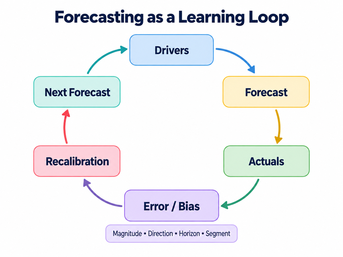
The next forecast is then generated from the revised mechanics:
Drivers → Forecast → Actuals → Error / Bias → Recalibration → Next Forecast
That loop offers traceability rather than a promise of ever-increasing accuracy. It records where the miss appeared, what the team changed and which assumptions now support the next decision.
Three checks before management relies on the number
A forecast can be reviewed quickly without inventing another scorecard. One useful place to start is the last miss. Learn asks whether the forecast origin was preserved and whether the error can be located by magnitude, direction, horizon and segment before tracing it to a driver, assumption, data issue or cadence decision.
Then inspect the current number. Explain asks whether revenue, cost and cash outputs can be traced back to meaningful drivers and visible assumptions. A chain that ends at “last year + 10%” gives management no mechanism to diagnose when the number moves.
The remaining test is time. Stay Current asks whether the horizon and refresh cadence match the pace of the decision. A hiring decision due within three months cannot wait for a six-month update cycle; a slow-moving assumption does not need to be rebuilt every week.
References
- AICPA & CIMA - Rolling Plans and Forecasts
- Institute of Management Accountants - Overcoming FP&A’s Biggest Challenge: Predicting the Future
- Institute of Management Accountants - Developing an Effective Managerial Costing Model
- ICAEW - 20 principles for good spreadsheet practice, 2024 edition
- Association for Financial Professionals - 8 Steps for Creating a Rolling Forecast
- Association for Financial Professionals - Implementing a Rolling Forecast: Success Factors and Pitfalls
- Hyndman & Athanasopoulos - Forecasting: Principles and Practice, Evaluating Point Forecast Accuracy
- Hyndman & Athanasopoulos - Time Series Cross-Validation
- Hyndman & Koehler - Another Look at Measures of Forecast Accuracy
- Hyndman & Athanasopoulos - Evaluating Distributional Forecast Accuracy
- GFOA - Planning and Budgeting Overview
- Federal Reserve Board / OCC - Supervisory Guidance on Model Risk Management
- Ekholm & Wallin - Is the Annual Budget Really Dead?