Customer B looks ordinary in a gross-margin report. Revenue is 100,000, COGS is 40,000 and gross profit is 60,000, exactly the same as Customer A.
The workload is not ordinary. B uses three times as many onboarding hours, three times as much support, more exception handling and more custom reporting. That difference only becomes visible once the management question changes. A gross-margin report can describe the accounting margin. It cannot, on its own, tell the company what will happen to resources or cash if B is repriced, redesigned or removed.
This article follows the same pair of customers through four views: reported gross margin, Cost-to-Serve, fully allocated profit and avoidable / incremental decision cost. Each view is useful. The error is to let one of them answer a question it was not built for.
Decide what the number is for
The four views can sit side by side:
| Cost lens | What it is mainly trying to answer | Common misuse |
|---|---|---|
| Gross Margin | What remains after the company’s defined COGS / cost-of-revenue boundary? | Treating gross margin as complete customer or product profitability |
| Cost-to-Serve | Which activities and resources does a customer, product, channel or service tier consume? | Treating every assigned cost as immediately cash-avoidable |
| Fully Allocated Profit | What does the cost object look like after shared or corporate costs are allocated? | Treating a negative allocated result as proof that exit creates value |
| Avoidable / Incremental Economics | If a specified action is taken over a specified horizon, which revenues, costs, cash flows and capacities actually change? | Looking only at short-term cash and ignoring opportunity cost or longer-run capacity release |
IMA’s managerial-costing guidance is useful here because it separates decision-useful costing from the cost model used for financial reporting. A management model needs to reflect the purpose of the decision and the causal consumption of resources. An allocated charge does not become avoidable simply because the report has assigned it to a customer. A pricing review, a 90-day keep-or-drop decision and long-run capacity planning can therefore use the same source data while drawing different cost boundaries. IMA: Developing an Effective Managerial Costing Model
Follow the work before judging the customer
Direct and indirect are properties of the relationship between a resource and a declared cost object. A resource can be direct to a product line yet require an activity driver when the object becomes an individual customer. IMA: Conceptual Framework for Managerial Costing
Activity-Based Costing makes that relationship explicit:
resources → activities → cost objects
For A and B, the synthetic activity data are:
| Activity | Rate | Customer A | A cost | Customer B | B cost |
|---|---|---|---|---|---|
| Implementation / onboarding | 100 / hour | 40 h | 4,000 | 120 h | 12,000 |
| Support | 50 / hour | 80 h | 4,000 | 240 h | 12,000 |
| Exception handling | 80 / case | 20 | 1,600 | 75 | 6,000 |
| Custom reporting / operations | 100 / hour | 20 h | 2,000 | 50 h | 5,000 |
| Cost-to-Serve | 11,600 | 35,000 |
The figures are illustrative units rather than observed company data. They change the customer view substantially: A moves from 60,000 gross profit to 48,400 after Cost-to-Serve, while B moves to 25,000.
- A: 60,000 − 11,600 = 48,400
- B: 60,000 − 35,000 = 25,000
The same modelling problem appears in businesses with very different operating drivers. Cloud costs may combine compute, tiering, egress and step pricing. Payments can depend on transaction counts, payment methods, cross-border activity, refunds and disputes. Communications services can include usage-linked network or carrier charges. Those examples are why a single average rate often hides the workload rather than explaining it. At this point B carries 35,000 of Cost-to-Serve, but the decision still depends on whether the underlying resources would disappear if B did. AWS EC2 Pricing Google Cloud Network Pricing Stripe Pricing
Capacity changes the keep-or-drop arithmetic
Kaplan and Anderson’s Time-Driven Activity-Based Costing uses two core estimates: the unit cost of supplying resource capacity, and the time or resource demand of each transaction or activity. Keeping those two estimates separate allows supplied, used and unused capacity to remain visible. Kaplan & Anderson, Time-Driven Activity-Based Costing
Take the support team. It supplies 2,500 hours of practical capacity for a period resource cost of 125,000, giving a capacity cost rate of 50 per hour. Current use is 2,250 hours, leaving 250 hours unused. B consumes 240 support hours, so the model assigns 12,000 of support capacity cost to B.
Removing B changes the utilisation profile, not necessarily the payroll. Used hours fall to 2,010 and unused capacity rises to 490:
| Support capacity | Before dropping B | After dropping B |
|---|---|---|
| Practical capacity | 2,500 h | 2,500 h |
| Used capacity | 2,250 h | 2,010 h |
| Unused capacity | 250 h | 490 h |
| Period resource cost | 125,000 | 125,000 |
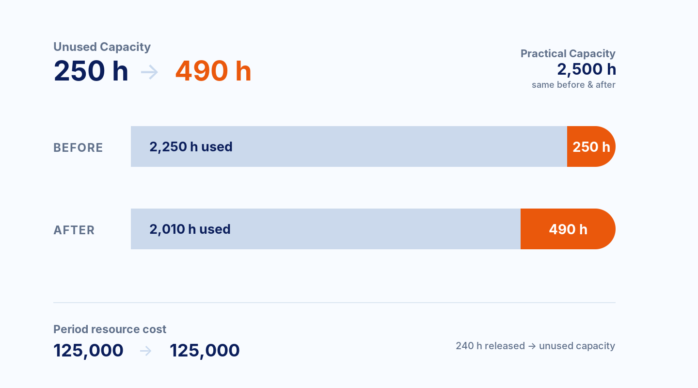
If the team is salaried and cannot be reduced over the decision horizon, period resource cost remains 125,000. The 12,000 assigned to B has moved from used capacity into unused capacity rather than becoming a cash saving. IAS 2 also uses a capacity concept, but for inventory costing and external reporting: its normal-capacity treatment limits the amount of fixed production overhead pushed into each unit during abnormally low production or idle plant. It does not set the managerial denominator for customer Cost-to-Serve. IAS 2 Inventories
A bottleneck creates a different problem
Spare support capacity does not create the same economics as a fully committed onboarding team. If implementation is the only genuinely binding resource and there is valuable alternative demand, each hour given to B has an opportunity cost.
For a single constrained resource, OpenStax uses contribution per unit of that resource as the comparison. OpenStax: Decisions When Resources Are Constrained Using implementation/onboarding hours as the sole constraint here:
- A: 60,000 − 4,000 support − 1,600 exceptions − 2,000 reporting = 52,400; over 40 implementation hours, that is 1,310 per constrained hour.
- B: 60,000 − 12,000 support − 6,000 exceptions − 5,000 reporting = 37,000; over 120 implementation hours, that is about 308.33 per constrained hour.
That result makes B expensive in scarce implementation capacity, but only under the stated conditions. If implementation is not binding, if there is no worthwhile alternative demand, or if several constraints and contractual obligations interact, the ratio is not a complete ranking rule.
Time determines how much cost can actually leave
A team can be fixed over one horizon and adjustable over another. Support might handle 10,000 to 12,000 tickets without hiring, add another team above that threshold, then retain the team for a while even after ticket volume falls. Cost behaviour therefore needs a driver, a relevant range and a time period. OpenStax: Cost Behaviour
The empirical cost-stickiness literature gives a useful warning against symmetrical assumptions. Anderson, Banker and Janakiraman studied 7,629 firms and found that, in their sample, SG&A rose by about 0.55% for a 1% rise in sales but fell by only about 0.35% for a 1% fall in sales. Those are sample findings, not universal forecasting coefficients. Anderson, Banker & Janakiraman, Are Selling, General, and Administrative Costs “Sticky”?
For B, a 90-day decision may leave almost all salaried support and implementation capacity in place. Over twelve months, attrition, hiring freezes, tooling changes, team consolidation or facilities decisions may release part of that capacity. The same assigned cost can therefore have very different avoidability depending on the horizon.
Read allocated profit as a signal, then test avoidability
Add corporate and shared-services cost to the customer report, allocated by revenue. A and B have equal revenue, so each receives 30,000:
| Lens | Customer A | Customer B |
|---|---|---|
| Gross Profit | 60,000 | 60,000 |
| Less Cost-to-Serve | (11,600) | (35,000) |
| Profit before shared allocation | 48,400 | 25,000 |
| Shared allocation | (30,000) | (30,000) |
| Fully Allocated Profit | 18,400 | (5,000) |
The fully allocated view has done something useful: it has identified B as a customer worth investigating. Pricing, support demand, service entitlements and custom work now deserve attention. The report has not yet shown that dropping B creates 5,000 of value.
For a 90-day keep-or-drop decision, the avoidability table looks different:
| B item | Assigned amount | 90-day avoidable cash |
|---|---|---|
| Implementation capacity | 12,000 | 0 |
| Support capacity | 12,000 | 0 |
| Outsourced exception handling | 6,000 | 6,000 |
| Custom reporting / operations capacity | 5,000 | 0 |
| Shared corporate allocation | 30,000 | 0 |
| Total immediately avoidable cost | 6,000 |
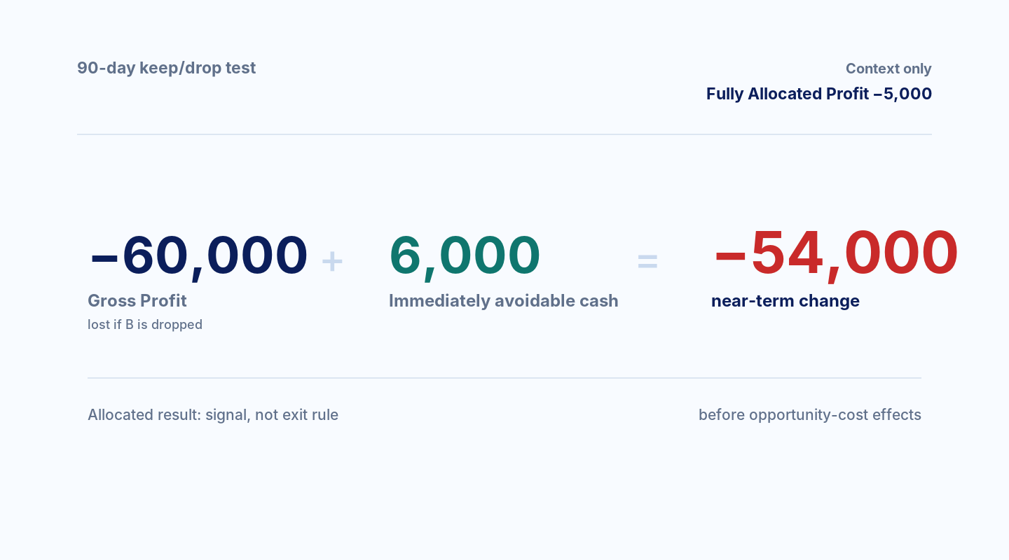
Removing B gives up 60,000 of gross profit and saves 6,000 of near-term cash cost. Before any opportunity-cost effects, the near-term change is −54,000. OpenStax’s keep-or-discontinue framework uses the same relevant-cost boundary: compare lost contribution with costs that are genuinely avoidable rather than with a fully allocated segment result. OpenStax: Keep or Discontinue
Allocation still has jobs to do. A managerial cost model may allocate for resource accountability or pricing discipline; external reporting follows its accounting framework; tax and transfer pricing use a separate arm’s-length framework for intra-group services. The allocation key should be read with that purpose attached.
OECD Transfer Pricing Guidelines Chapter VII, for example, discusses consistent allocation keys for low-value intra-group services that reflect the nature of the service and expected benefit. Depending on the service, examples include headcount, users, vehicles, transactions or assets. This is useful evidence for disciplined allocation design, while remaining tax transfer-pricing guidance rather than a universal rule for internal managerial costing. OECD Transfer Pricing Guidelines 2022
Reconcile period changes before explaining them
Suppose customer profitability falls next quarter. A bridge can first reconcile the movement across volume or customer count, customer or service mix, Cost-to-Serve intensity, capacity utilisation, and relevant FX, scope, timing or allocation-method changes. The method and cost-object definitions need to stay stable, and the components should add from the starting total to the ending total.
That produces arithmetic attribution, not causal proof. If support hours and customer mix both move, the bridge can show how much each contributes to the reported change. Evidence about the business mechanism still has to come from elsewhere.
Work the levers before the exit decision
Under the current 90-day assumptions, the avoidable-cost arithmetic does not support an immediate exit. Management can work the case in a much smaller loop.
First, fix the decision and horizon. If the question is renewal or pricing, analyse B as a customer; if the question is capacity planning, identify the resource that is actually constrained. Then use the Cost-to-Serve detail to target the workload that can change: onboarding, support, exception handling or custom reporting. Finally, separate resources that can be released from capacity that would merely become idle, and add opportunity cost only where a genuine bottleneck and worthwhile alternative demand exist.
That leaves several practical actions before termination: reprice B, reduce exception demand, standardise custom reporting, redesign onboarding or support, or redeploy scarce implementation capacity. A longer horizon may eventually make support, implementation or shared capacity removable. If it does, rerun the economics with that new horizon rather than extending the 90-day answer by assumption.
The allocation key should also remain labelled with its purpose. A key designed for accountability, pricing discipline, external reporting or tax compliance can inform the decision without being allowed to decide it automatically.
What would actually change if B left?
B’s Fully Allocated Profit is −5,000. Its currently modelled 90-day avoidable cash is only 6,000. Those figures can coexist because they answer different questions.
For the exit decision, the remaining tests are concrete: which resources and cash flows change within the chosen horizon, whether a real bottleneck creates opportunity cost, and whether any capacity can actually be released. Until those conditions change, the allocated loss is a warning to investigate, not proof that exit creates value.
References
- IMA, Conceptual Framework for Managerial Costing
- IMA, Developing an Effective Managerial Costing Model
- Robert S. Kaplan and Steven R. Anderson, Time-Driven Activity-Based Costing
- Harvard Business School Working Knowledge, Adding Time to Activity-Based Costing
- OpenStax, Identify and Apply Basic Cost Behavior Patterns
- OpenStax, Evaluate and Determine Whether to Keep or Discontinue a Segment or Product
- OpenStax, Evaluate and Determine How to Make Decisions When Resources Are Constrained
- Mark C. Anderson, Rajiv D. Banker and Surya N. Janakiraman, Are Selling, General, and Administrative Costs “Sticky”?
- IFRS Foundation, IAS 2 Inventories
- OECD, OECD Transfer Pricing Guidelines for Multinational Enterprises and Tax Administrations 2022
- AWS, EC2 On-Demand Pricing
- Google Cloud, VPC Network Pricing
- Stripe, Pricing