A market-sizing slide can be perfectly correct arithmetically and still be useless for a decision.
Take the familiar line: “The market is US100 million.” The multiplication works. What has not been shown is whether that 1% refers to eligible customers, adoption in the planning period, commercial reach, competitive wins, delivery capacity, or the share of market activity that the company can actually monetise.
One percentage has been asked to do six different jobs.
The better question is not “How large can we make TAM?” It is “What must be true at every step between the market and company revenue?” That is the organising idea for the model below.
Start with the denominator, not the headline number
Before calculating TAM, write down what the number is supposed to measure. A practical Market Sizing Measurement Contract should fix the economic unit, product or job boundary, eligible customer population, geography, time horizon, price or currency basis, source period, and whether the starting figure represents industry activity or company revenue.
That sounds administrative, but it prevents some of the largest errors in the model. A market measured in software spend is not automatically the same market as a population of eligible organisations. A global industry total cannot be carried into a regional go-to-market model without showing what has been removed. A transaction-value denominator cannot quietly become recognised revenue halfway through the calculation.
The SBA separates questions such as demand, market size, location, saturation and pricing in market research. US merger guidance uses product and geographic boundaries to analyse substitution and competitive constraints. Neither is a universal TAM formula, but both reinforce the same discipline: the boundary comes before the number.
For a regional compliance-workflow product, “all enterprise software spend” may be a useful context statistic and a poor denominator. The relevant universe could be restricted by regulation, workflow, company size, implementation requirements and geography long before any market-share assumption is introduced.
Make top-down and bottom-up disagree in useful ways
Suppose an adjacent industry-spend source suggests US$1.2 billion. That is a top-down observation, not yet the target market.
Now build a separate bottom-up view. Assume there are 20,000 potential organisations in the broad target universe and use US200 million.
Those figures are not close, and that is useful. Averaging them to US$700 million would erase the very information we need to investigate.
The reconciliation should ask, for example:
- Does the US$1.2 billion include adjacent categories that the product does not address?
- Are the two estimates counting the same economic unit, or is one closer to supplier revenue while the other reflects end-customer value?
- Does the industry total contain double counting across a supply chain?
- Are geography and customer eligibility aligned?
- Is US$10,000 a realised price, an ACV assumption, a value proxy or a willingness-to-pay estimate?
County Business Patterns can help test establishment populations by geography and industry. BEA’s distinction between gross output and value added is a useful reminder that large aggregates can describe different layers of economic activity. These sources help us interrogate the denominator; they do not relieve us of the reconciliation work.
If part of the US200 million gap remains unexplained, keep the residual visible. An unresolved difference is a finding, not a rounding problem.
Treat TAM, SAM and SOM as constraints with a clock
The usual three-circle diagram becomes more useful when each narrowing has a named reason.
A workable sequence is:
Defined TAM → Serviceable SAM → Adoption within the horizon → Commercial reach → Attainable share / SOM
Defined TAM is the complete demand universe inside the measurement contract. Serviceable SAM removes customers the current offer cannot serve because of product, technical, legal, geographic or commercial constraints.
Then time enters the model. A customer can belong to the market and still have no intention of adopting in the next twelve or twenty-four months. Bass diffusion is relevant here only as evidence that adoption can be modelled as a population process over time. It is not a licence to impose one S-curve on every market.
Reach is a different filter again. Distribution, sales coverage, partners, procurement access and channel economics determine which potential adopters the company can actually engage. Only after those filters does competitive share become meaningful.
This is why “SAM is 30% of TAM, then SOM is 1%” is not a method unless the percentages correspond to documented constraints.
A worked B2B case: from broad opportunity to near-term revenue
Use the bottom-up case as a teaching model, with every input explicitly hypothetical and not a benchmark.
The broad universe contains 20,000 organisations. Product, geography and eligibility rules reduce the serviceable population to 7,500. On the same US75 million** of value, but it is still not a revenue forecast.
Now add the time and execution filters:
| Filter | Assumption | Remaining organisations |
|---|---|---|
| Serviceable population | fixed by product / geography / eligibility | 7,500 |
| Adoption in the planning horizon | 35% | 2,625 |
| Commercial reach among adopters | 60% | 1,575 |
| Attainable competitive share | 20% | 315 |
At this point the model has 315 demand-derived customers. With an illustrative US$10,000 ACV, that becomes:
315 × US3.15 million annual revenue opportunity before capacity
Each multiplier has a different owner and a different evidence burden. Serviceability is a product and market-boundary question. Adoption is a timing question. Reach belongs to the distribution system. The 20% share assumption needs competitive and conversion evidence.
The top-down US$1.2 billion figure still exists in the analysis, but it is not averaged into this result. Its role is to challenge the bottom-up boundary and expose any missing category or unit mismatch.
There is one more constraint. If sales, implementation and onboarding can support only 300 new customers in the same period, the near-term ceiling is:
300 × US3.0 million
Demand supports 315 wins; the operating system can absorb 300. That fifteen-customer gap is an execution constraint, not evidence that the underlying demand vanished.
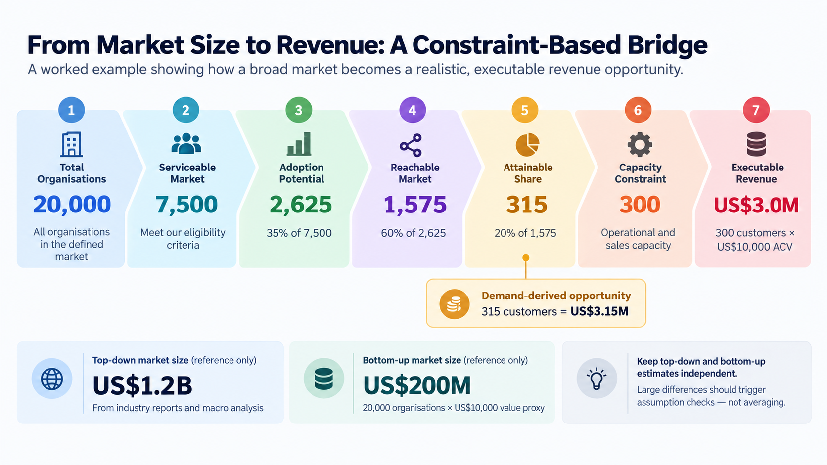
The Top-down US3.15M opportunity to a capacity-capped US$3.0M executable opportunity.
Market activity still has to cross the monetisation bridge
Customer × ACV makes the worked example unusually clean. Other business models start from denominators that are much further away from revenue.
Marketplaces and payments businesses may describe activity through GMV, GBV, TPV, GOV, payments volume, transactions or gross bookings. These measures can be central to the business and still not be revenue. Airbnb reports booking value separately from revenue. Visa distinguishes payments volume and processed transactions from net revenue. eBay’s take-rate calculation requires an aligned relationship between net revenue and GMV. DoorDash similarly connects marketplace GOV to monetisation through revenue margin rather than treating GOV as sales.
The key drafting question is therefore: what event or economic unit actually triggers revenue for this company?
For recurring software, eligible customers multiplied by effective ACV may be sufficient. For a marketplace, eligible transaction value may need a realised take rate. Payments models can require transaction counts, volume, cross-border mix, product mix and fee structure. Booking Holdings also shows how payment facilitation, product mix and the timing between booking and travel can affect the bridge from activity to reported revenue.
A useful synthesis is:
Revenue Opportunityₜ ≈ Eligible Economic Units × Adoptionₜ × Reachₜ × Attainable Shareₜ × Usageₜ × Effective Monetisationₜ
It is a teaching scaffold, not a universal equation. The driver set should change with the business model. What should not change silently is the denominator between the market side and the company-revenue side.
When demand is larger than the system that has to serve it
Capacity deserves its own line in the model because hiding it inside market share makes the diagnosis worse.
In the worked example, 315 customers are demand-derived and 300 are capacity-capped. A management team looking only at the first number could spend against demand that the organisation cannot onboard in the period. A team looking only at the second could miss the fact that there is already excess demand worth unlocking through more implementation or sales capacity.
The binding constraint can be rep ramp time, partner coverage, implementation staff, inventory, regulated approvals, geographic operations, support throughput or risk-control capacity. The right capacity model depends on the business.
Keep two ceilings visible:
Demand-derived attainable opportunity
Execution / channel / capacity ceiling
The lower one governs the near-term result. The gap between them tells you which system has to change next.
Multi-sided markets require a related discipline. Buyers and sellers, or cardholders and merchants, are not interchangeable revenue units. Adding populations from both sides and multiplying by one ARPU can double count participation and apply the wrong monetisation basis. Define the side, event and denominator on which the company actually earns money.
Finish with a switching value, not a more decorative forecast
Once the chain is explicit, sensitivity analysis becomes more useful than another point estimate.
The base case contains a simple switching value. Keep serviceable population at 7,500, reach at 60% and attainable share at 20%. Capacity is 300 customers. The adoption rate at which demand exactly meets capacity is:
7,500 × adoption × 60% × 20% = 300
That gives an adoption threshold of about 33.3%.
Above that level, the 300-customer capacity ceiling binds first. Below it, demand becomes the limiting factor.
If adoption falls to 25%, the model produces:
7,500 × 25% × 60% × 20% = 225 customers
225 × US2.25 million
The decision implication changes. Adding onboarding capacity is no longer the first priority; improving the adoption evidence or the product’s ability to move that assumption becomes more important.
NIST’s treatment of measurement uncertainty is useful here as a methodological analogy: expose the components rather than burying them in one number. HM Treasury’s Green Book uses sensitivity and switching values in appraisal for a similar reason. Neither source turns market sizing into a physical measurement exercise; both support the discipline of showing what can change the decision.
Low, Base and High cases can still be useful. They should not be assigned pseudo-probabilities unless the analyst has evidence for the underlying distribution or priors.
Before a market-sizing model is used for investment, product or go-to-market decisions, it should answer four questions:
- Boundary: what people, products, transactions and geographies are actually included?
- Bridge: how does the market denominator become company revenue?
- Constraint: which of adoption, reach, competition, channel or capacity currently controls the result?
- Switching value: how far must a key assumption move before the decision changes?
Those answers make the opportunity auditable, and they tell the team what evidence to collect next.
References
- U.S. Small Business Administration, Market research and competitive analysis.
- U.S. Department of Justice, 2023 Merger Guidelines, with market-definition concepts used here only as boundary discipline.
- U.S. Census Bureau, County Business Patterns: About the Data.
- U.S. Bureau of Economic Analysis, GDP by Industry and Gross output versus GDP by industry.
- Frank M. Bass, A New Product Growth for Model Consumer Durables, Management Science (1969).
- Airbnb, Inc., 2025 Form 10-K.
- Visa Inc., 2025 Annual Report.
- eBay Inc., 2024 Form 10-K.
- DoorDash, Inc., Q1 2025 Financial Results.
- Booking Holdings Inc., Q1 2026 Form 10-Q.
- NIST, Technical Note 1297: Guidelines for Evaluating and Expressing the Uncertainty of NIST Measurement Results.
- HM Treasury, The Green Book: Central Government Guidance on Appraisal and Evaluation.