Three reasonable ranges before the valuation meeting has even started
Imagine a fictional company, Northstar Co., with two very different businesses. Segment A sells subscription software with steadier revenue and higher margins. Segment B runs a transaction platform whose growth depends more heavily on volume, take rate and market cycles.
The valuation work produces three enterprise-value ranges:
| Method | Illustrative Northstar EV range |
|---|---|
| DCF | 400–515 |
| Trading multiples | 455–535 |
| SOTP | 465–550 |
The meeting now has a problem. The numbers overlap, but they do not agree. Averaging the midpoints would make the slide cleaner without explaining any of the difference. Choosing one model as the answer and demoting the others to cross-checks can hide the same issue.
Each method carries a different set of assumptions. DCF turns expected cash flows and discounting into present value. Trading multiples import the market’s pricing of a chosen peer group. SOTP allows separate businesses to use separate valuation lenses. The distance between the ranges can therefore reveal something about the assumptions rather than merely creating noise.
Before deciding how much confidence to place in any range, Northstar needs two controls: every method must value the same claim, and each method must be internally coherent.
Put every result on the same claim first
Valuation outputs commonly sit at four different levels:
| Layer | What it measures |
|---|---|
| Segment value | One business or asset |
| Enterprise value | The operating business for all capital providers |
| Equity value | The value attributable to shareholders after bridge items |
| Per-share value | Equity value divided by the relevant diluted share count |
Northstar labels the initial DCF, trading-multiple and SOTP outputs as enterprise value. That labelling matters because a comparison can otherwise mix financing layers without making the mismatch visible.
Take a 12x EV/EBITDA calculation and a P/E calculation. The first starts with enterprise value and an operating denominator before interest. P/E is already an equity-level measure. A valuation table can calculate both correctly and still compare unlike claims.
The same applies to DCF. Northstar discounts unlevered free cash flow, so the result stays at enterprise level. A DCF built from cash flow available to equity holders would land elsewhere. The model name alone does not identify the claim.
Once the claim level is fixed, differences between methods become much easier to interpret. Until then, a spread can be nothing more than a missing bridge.
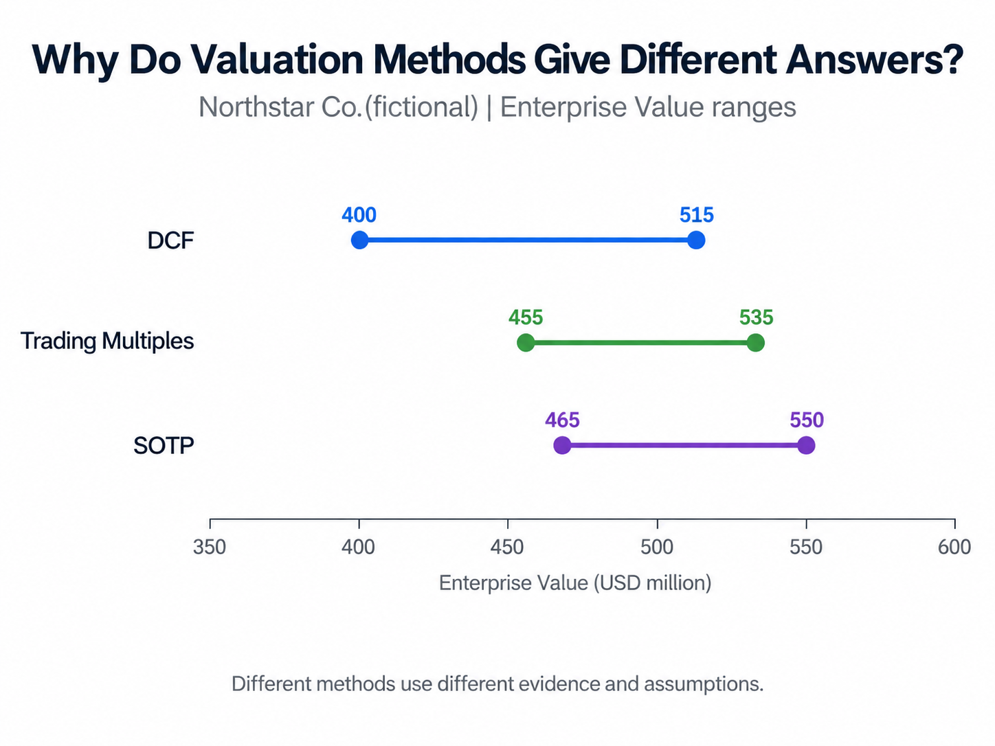
All three methods are shown at Enterprise Value; the methods use different evidence and assumptions.
Review the DCF through its connections
A simplified unlevered DCF for Northstar is straightforward:
Enterprise Value
= PV of unlevered free cash flow during the explicit forecast period
+ PV of terminal value
The spreadsheet can execute that expression perfectly while the economics underneath it remain inconsistent. A useful review therefore follows the connections between inputs.
Northstar’s unlevered cash flow needs a discount rate appropriate to enterprise-level cash flows. The currency basis also needs to match: nominal US-dollar cash flows should use a risk-free foundation consistent with those dollar cash flows.
Terminal value deserves a separate read. A perpetual-growth terminal value rests on long-run growth and mature economics. An exit-multiple terminal value brings market-relative evidence into the final stage of the model. Both can be used in practice, but a reviewer should know which source of value is carrying the result.
For the base case, assume WACC is 9.5% and terminal growth is 2.5%. The model produces an EV of about 440. Moving those assumptions gives the following grid:
| Terminal growth / WACC | 8.5% | 9.5% | 10.5% |
|---|---|---|---|
| 2.0% | 470 | 430 | 397 |
| 2.5% | 490 | 440 | 405 |
| 3.0% | 515 | 455 | 416 |
This is a sensitivity table. It shows how strongly the DCF responds to WACC and long-run growth; it does not assign a probability to each cell or turn 440 into an expected value.
A second layer of review concerns the forecast itself. Growth eventually has to meet a credible mature-state margin. Nominal cash flow should be paired with nominal discounting. A risk already reflected in lower cash flow should not quietly receive another full penalty in the discount rate. These checks can change the valuation even when every formula in the workbook is syntactically correct.
For Northstar, the DCF is useful because the cash-flow assumptions are visible and challengeable. Its main weakness is equally visible: terminal value and discount-rate assumptions can move the range materially.
Trading multiples inherit every choice in the peer set
A comps page often looks more empirical than a DCF because it begins with observed market prices. The judgement has simply moved to a different place.
Suppose Northstar starts with a broad peer group covering software and platform companies. That set might imply 520–610 EV. Tightening the group around companies with more comparable revenue mix, growth and margin profiles pulls the illustrative range down to 455–535.
Nothing in the multiplication changed. The reference set did.
Industry labels alone are rarely enough. Growth, gross margin, retention, capital intensity, customer concentration, scale, cyclicality and revenue quality can all affect the multiple investors are willing to pay. In In re Appraisal of SWS Group, the Delaware Court of Chancery rejected a comparable-company analysis where size and business differences undermined reliability. The case is useful here as a boundary: comparability needs economic support.
The denominator requires the same discipline. EV/EBITDA belongs at enterprise level; P/E belongs at equity level. One-off items, accounting differences or abnormal margins may also require normalisation before Northstar is compared with the peer set.
A reviewer should therefore be able to trace a trading-multiple result back to the companies selected, the reason they belong in the set, the multiple used and the financial metric to which it was applied. The 455–535 range is only as useful as that chain.
Split the businesses, then bring the results back to equity value
Segment A and Segment B do not share the same economics. A single consolidated EV/EBITDA multiple would flatten subscription software and a transaction marketplace into one average, so Northstar uses SOTP to value them separately.
| Segment | Illustrative valuation lens | Illustrative EV |
|---|---|---|
| A: subscription software | Relevant subscription peers plus cash-flow cross-check | 330–385 |
| B: transaction platform | Marketplace peers plus profitability adjustment | 135–165 |
| SOTP total | 465–550 |
The benefit is visible in the inputs. Each segment can use a reference set that fits its own economics. The cost is higher dependence on segment reporting and segment-level peer quality.
No conglomerate discount is added. The existence of two segments does not establish a discount or its size, and it would be equally weak to subtract 10% simply because a spreadsheet has a row available for it. A separate adjustment would need separate evidence about governance, capital allocation, disclosure or market structure.
Northstar now has three enterprise-value ranges, but shareholders hold the equity claim. Assume debt of 80 and excess cash of 30. Preferred claims, minority interests, convertibles, options and complex diluted-share mechanics stay outside the fictional case.
Equity Value = Enterprise Value - Debt + Excess CashThe net bridge is -50.
| Method | EV range | EV→Equity adjustment | Equity-value range |
|---|---|---|---|
| DCF | 400–515 | -50 | 350–465 |
| Trading multiples | 455–535 | -50 | 405–485 |
| SOTP | 465–550 | -50 | 415–500 |
Real companies can add debt-like liabilities, non-operating assets, minority interests, preferred claims or pension deficits to that bridge. The relevant set depends on the company and the purpose of the valuation. For comparison, every bridge item needs a definition and every method needs the same valuation date and claim level.
Read sensitivity as a map of where the DCF can move
The earlier grid moved WACC from 8.5% to 10.5% and terminal growth from 2.0% to 3.0%, taking illustrative EV from about 397 to 515. The review implication is practical: challenge the assumptions with enough leverage to change the result.
Two-way sensitivity can also be used elsewhere, for example multiple × normalised EBITDA in relative valuation. A grid still says nothing about probability unless a separate scenario or probabilistic model supplies it.
At this stage Northstar’s differences are traceable. DCF is close to the company’s own cash-flow forecast but sensitive to long-run assumptions. Trading multiples inherit the quality of the peer set. SOTP fits the two-engine business model but needs credible segment data. The common bridge has removed the EV/equity mismatch.
Reconciliation should leave a trail another reviewer can challenge
Put the three equity ranges next to their strongest support and their main limitation:
| Method | Equity-value range | Strongest support | Main limitation |
|---|---|---|---|
| DCF | 350–465 | Direct link to company cash flow and long-run economics | Terminal value and WACC sensitivity |
| Trading multiples | 405–485 | Observable market pricing and relative benchmarks | Peer selection and normalisation |
| SOTP | 415–500 | Separates two distinct business engines | Segment data and segment-level peer quality |
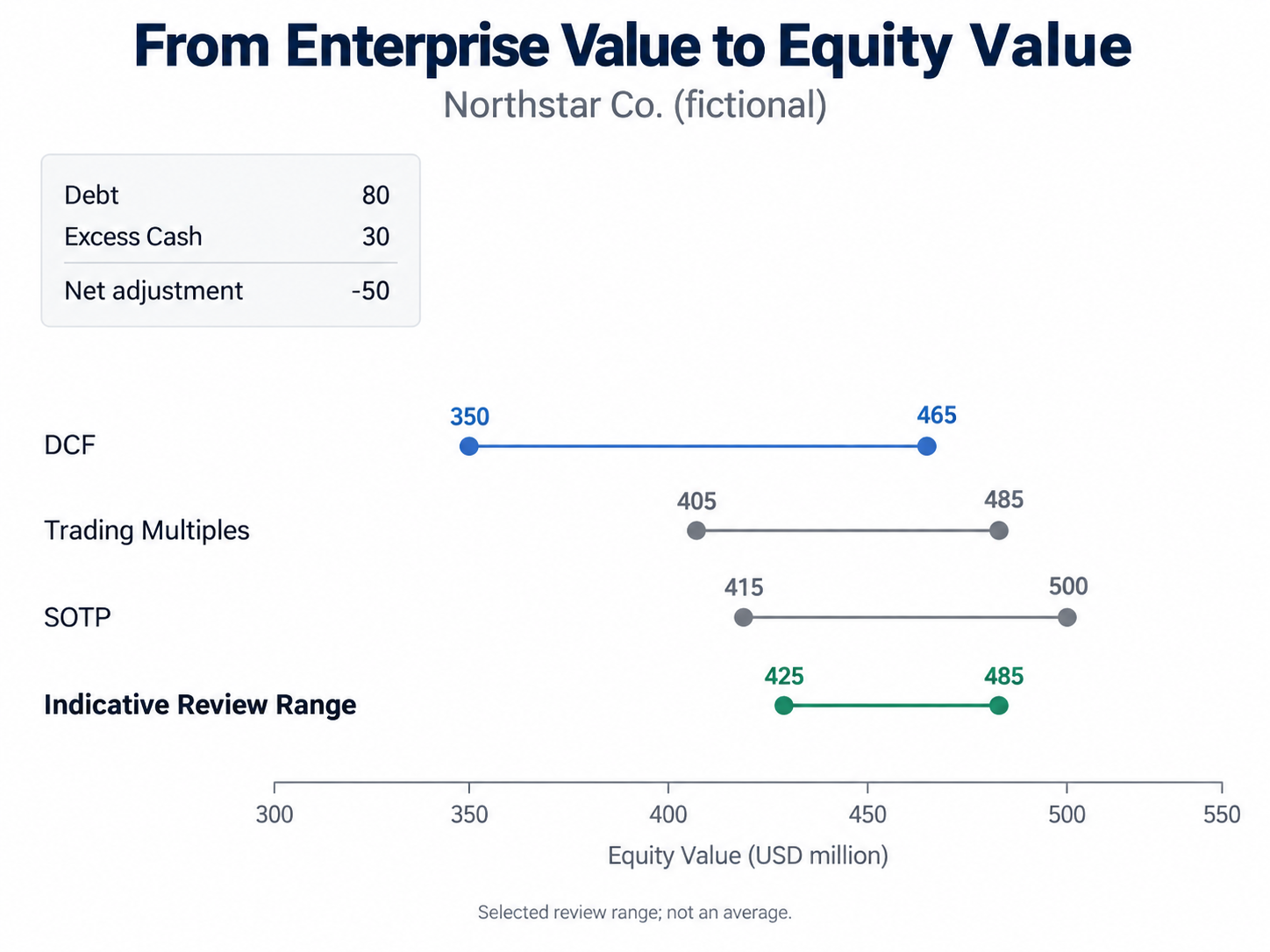
After normalization to Equity Value, the Illustrative Core Range of 425–485 is a selected review range, not a mechanical average, confidence interval, or expected value.
The simple intersection is roughly 415–465. There is no requirement for the final range to stop there.
If Northstar has excellent segment reporting and clean segment peers while terminal value dominates its DCF, SOTP and trading multiples may carry more weight in the discussion. If the peer set comes from a euphoric market period and Northstar has well-supported mature cash flows, the balance can move back towards DCF.
For this fictional teaching case, 425–485 is an intentionally selected illustrative core equity-value range. It preserves the information from DCF sensitivity, peer quality, SOTP business fit and the common EV-to-equity bridge. There is no unique formula that derives 425–485 from the three preceding ranges, and the number should not be read as a statistical confidence interval.
Transaction evidence can be added when it is relevant. DFC Global Corp. v. Muirfield Value Partners shows why deal price can carry substantial information when the market check and surrounding facts support it. Different timing, control rights, transaction structures or sale processes can reduce that comparability. A realised price belongs in the evidence set with those conditions attached.
Strategic value and synergy stay outside Northstar’s base case. Claims about acquisition synergies, control value or deal-specific economics need transaction-level evidence and their own modelling. That work belongs in the deeper M&A and corporate-development analysis.
The useful output of reconciliation is therefore a reviewable judgement: another analyst should be able to identify which peer, assumption, segment lens or bridge item they would change, and explain how that change moves the range. If the range cannot be challenged at that level, the model has produced a number without producing much understanding. A spreadsheet ending at 472.6 does not solve that review problem.
References
- Aswath Damodaran, NYU Stern, An Introduction to Valuation.
- Aswath Damodaran, NYU Stern, Terminal Value.
- Aswath Damodaran, NYU Stern, Estimating Risk Free Rates.
- CFA Institute Research Foundation, Equity Valuation: Science, Art, or Craft?.
- CFA Institute, Market-Based Valuation: Price and Enterprise Value Multiples.
- FactSet, market and enterprise value methodology materials.
- International Valuation Standards Council, What IVS Asks of Every Business Valuation.
- U.S. Securities and Exchange Commission, K2 / Blackstone merger proxy (2007), DCF architecture example.
- U.S. Securities and Exchange Commission, Norfolk Southern / BofA financial analysis (2025), WACC-range DCF example.
- U.S. Securities and Exchange Commission, DecisionPoint / Craig-Hallum financial analysis (2024), transaction and terminal-multiple example.
- Delaware Court of Chancery, In re Appraisal of SWS Group.
- Delaware Supreme Court, DFC Global Corp. v. Muirfield Value Partners.
- Cornerstone Research, Appraisal Litigation in Delaware: 2006–2022.
- European Commission Joint Research Centre, sensitivity-analysis guidance.
- HM Treasury, appraisal-calculation examples.